False-positive risk (power loss) when adding a futility interim analysis to a clinical trial

Purpose of this document

This R markdown file accompanies this linkedin post, provides the code to reproduce computations, and much more. I also talked about this topic at the first 2024 effective statistician conference, find my slides here

Acknowldegments

I talk(ed) a lot about this broad topic with my Roche colleagues Marcel Wolbers, Jenny Devenport, Gian Thanei, Jianmei Wang, Gaelle Klingelschmitt, Uli Burger, and many others.

Setup and definition of functions

We define a few hand-knitted functions to simulate clinical trials. I am sure there would be off-the-shelf methods for this, but I simply reuse what I have already.

library(survival)
library(rpact)

Installation qualification for rpact 4.4.0 has not yet been performed.

Please run testPackage() before using the package in GxP relevant environments.

library(reporttools)

Lade nötiges Paket: xtable

# Quantile function for a Weibull distribution with a cure proportion
qWeibullCure <- function(p, p0, shape = 1, scale){
  res <- rep(NA, length(p))
  ind1 <- (p <= p0)
  ind2 <- (p > p0)
  res[ind1] <- Inf
  res[ind2] <- qweibull(1 - (p[ind2] - p0) / (1 - p0), shape = shape, scale = scale)
  return(res)  
}

# censored time-to-event data with censoring after pre-specified number of events
rWeibull1arm <- function(shape = 1, scale, cure = 0, recruit, dropout = 0, start.accrual = 0, cutoff, seed = NA){
  
  # shape             Weibull shape parameter. 
  # scale:            Weibull scale parameter
  # cure:             Proportion of patients assumed to be cured, i.e. with an event at +infty.
  # recruit:          Recruitment.
  # dropout:          Drop-out rate, on same time scale as med.
  # start.accrual:    Time unit where accrual should start. Might be useful when simulating multi-stage trials.
  # cutoff:           Cutoff, #events the final censored data should have (can be a vector of multiple cutoffs).
  # seed:             If different from NA, seed used to generate random numbers.
  #
  # Kaspar Rufibach, June 2014
  
  if (is.na(seed) == FALSE){set.seed(seed)}
  
  n <- sum(recruit)
  
  # generate arrival times
  arrive <- rep(1:length(recruit), times = recruit)
  arrivetime <- NULL
  for (i in 1:n){arrivetime[i] <- runif(1, min = arrive[i] - 1, max = arrive[i])}
  arrivetime <- start.accrual + sort(arrivetime)
  
  # generate event times: Exp(lambda) = Weibull(shape = 1, scale = 1 / lambda)
  eventtime <- qWeibullCure(runif(n), p0 = cure, shape = shape, scale = scale)
  
  # Apply drop-out. Do this before applying the cutoff below, in order to correctly count necessary #events.
  dropouttime <- rep(Inf, n)
  if (dropout > 0){dropouttime <- rexp(n, rate = dropout)}
  event.dropout <- ifelse(eventtime > dropouttime, 0, 1)
  time.dropout <- ifelse(event.dropout == 1, eventtime, dropouttime)   
  
  # observed times, taking into account staggered entry
  tottime <- arrivetime + eventtime
  
  # find cutoff based on number of targeted events
  # only look among patients that are not considered dropped-out
  time <- data.frame(matrix(NA, ncol = length(cutoff), nrow = n))
  event <- time
  cutoff.time <- rep(NA, length(cutoff))
  
  for (j in 1:length(cutoff)){
    cutoff.time[j] <- sort(tottime[event.dropout == 1])[cutoff[j]]
    
    # apply administrative censoring at cutoff
    event[event.dropout == 1, j] <- ifelse(tottime[event.dropout == 1] > cutoff.time[j], 0, 1)
    event[event.dropout == 0, j] <- 0
    
    # define time to event, taking into account both types of censoring
    time[event.dropout == 1, j] <- ifelse(event[, j] == 1, eventtime, cutoff.time[j] - arrivetime)[event.dropout == 1]    # same as: pmin(tottime, cutoff.time) - arrive
    time[event.dropout == 0, j] <- pmin(cutoff.time[j] - arrivetime, time.dropout)[event.dropout == 0]
    
    # remove times for patients arriving after the cutoff
    rem <- (arrivetime > cutoff.time[j])
    if (TRUE %in% rem){time[rem, j] <- NA}
  }
  
  # generate output
  tab <- data.frame(cbind(1:n, arrivetime, eventtime, tottime, dropouttime, time, event))
  colnames(tab) <- c("pat", "arrivetime", "eventtime", "tottime", "dropouttime", paste("time cutoff = ", cutoff, sep = ""), paste("event cutoff = ", cutoff, sep = ""))
  
  res <- list("cutoff.time" = cutoff.time, "tab" = tab)
  return(res)
}

# censored time-to-event data with censoring after pre-specified number of events, for two treatment arms
rWeibull2arm <- function(shape = c(1, 1), scale, cure = c(0, 0), recruit, dropout = c(0, 0), start.accrual = c(0, 0), cutoff, seed = NA){
  
  # shape             2-d vector of Weibull shape parameter. 
  # scale             2-d vector of Weibull scale parameter.
  # cure:             2-d vector with cure proportion assumed in each arm.
  # recruit:          List with two elements, vector of recruitment in each arm.
  # dropout:          2-d vector with drop-out rate for each arm, on same time scale as med.
  # start.accrual:    2-d vector of time when accrual should start. Might be useful when simulating multi-stage trials.
  # cutoff:           Cutoff, #events the final censored data should have (can be a vector of multiple cutoffs).
  # seed:             If different from NA, seed used to generate random numbers.
  #
  # Kaspar Rufibach, June 2014
  
  if (is.na(seed) == FALSE){set.seed(seed)}
  
  dat1 <- rWeibull1arm(scale = scale[1], shape = shape[1], recruit = recruit[[1]], cutoff = 1, 
                                      dropout = dropout[1], cure = cure[1], start.accrual = start.accrual[1], seed = NA)$tab
  dat2 <- rWeibull1arm(scale = scale[2], shape = shape[2], recruit = recruit[[2]], cutoff = 1, 
                                      dropout = dropout[2], cure = cure[2], start.accrual = start.accrual[2], seed = NA)$tab
  
  n <- c(nrow(dat1), nrow(dat2))
  
  # treatment variable
  tmt <- factor(c(rep(0, n[1]), rep(1, n[2])), levels = 0:1, labels = c("A", "B"))
  
  arrivetime <- c(dat1[, "arrivetime"], dat2[, "arrivetime"])
  eventtime <- c(dat1[, "eventtime"], dat2[, "eventtime"])
  tottime <- c(dat1[, "tottime"], dat2[, "tottime"])
  dropouttime <- c(dat1[, "dropouttime"], dat2[, "dropouttime"])
  
  # Apply drop-out. Do this before applying the cutoff below, in order to correctly count necessary #events.
  event.dropout <- ifelse(eventtime > dropouttime, 0, 1)
  time.dropout <- ifelse(event.dropout == 1, eventtime, dropouttime)   
  
  # find cutoff based on number of targeted events
  # only look among patients that are not considered dropped-out
  time <- data.frame(matrix(NA, ncol = length(cutoff), nrow = sum(n)))
  event <- time
  cutoff.time <- rep(NA, length(cutoff))
  
  for (j in 1:length(cutoff)){
    cutoff.time[j] <- sort(tottime[event.dropout == 1])[cutoff[j]]
    
    # apply administrative censoring at cutoff
    event[event.dropout == 1, j] <- ifelse(tottime[event.dropout == 1] > cutoff.time[j], 0, 1)
    event[event.dropout == 0, j] <- 0
    
    # define time to event, taking into account both types of censoring
    time[event.dropout == 1, j] <- ifelse(event[, j] == 1, eventtime, cutoff.time[j] - arrivetime)[event.dropout == 1]    
    time[event.dropout == 0, j] <- pmin(cutoff.time[j] - arrivetime, time.dropout)[event.dropout == 0]
    
    # remove times for patients arriving after the cutoff
    rem <- (arrivetime > cutoff.time[j])
    if (TRUE %in% rem){time[rem, j] <- NA}
  }
  
  # generate output
  tab <- data.frame(cbind(1:sum(n), tmt, arrivetime, eventtime, tottime, dropouttime, time, event))
  colnames(tab) <- c("pat", "tmt", "arrivetime", "eventtime", "tottime", "dropouttime", 
                     paste("time cutoff = ", cutoff, sep = ""), paste("event cutoff = ", cutoff, sep = ""))

  res <- list("cutoff.time" = cutoff.time, "tab" = tab)
  return(res)
}

# functions to plot results
horiz <- function(vert = FALSE){
  segments(0, 1, 1, 1, col = 5, lwd = 4, lty = 1)
  segments(0, hr, 1, hr, col = 4, lwd = 4, lty = 1)
  segments(0, mdd_no_interim, 1, mdd_no_interim, col = 2, lwd = 4, lty = 1)
  
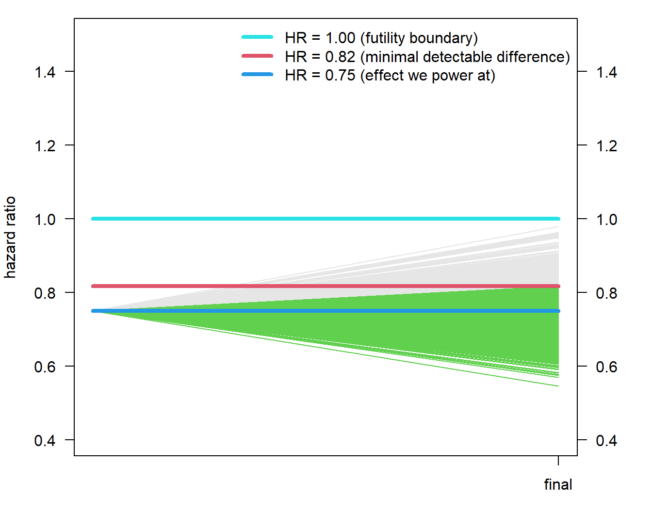
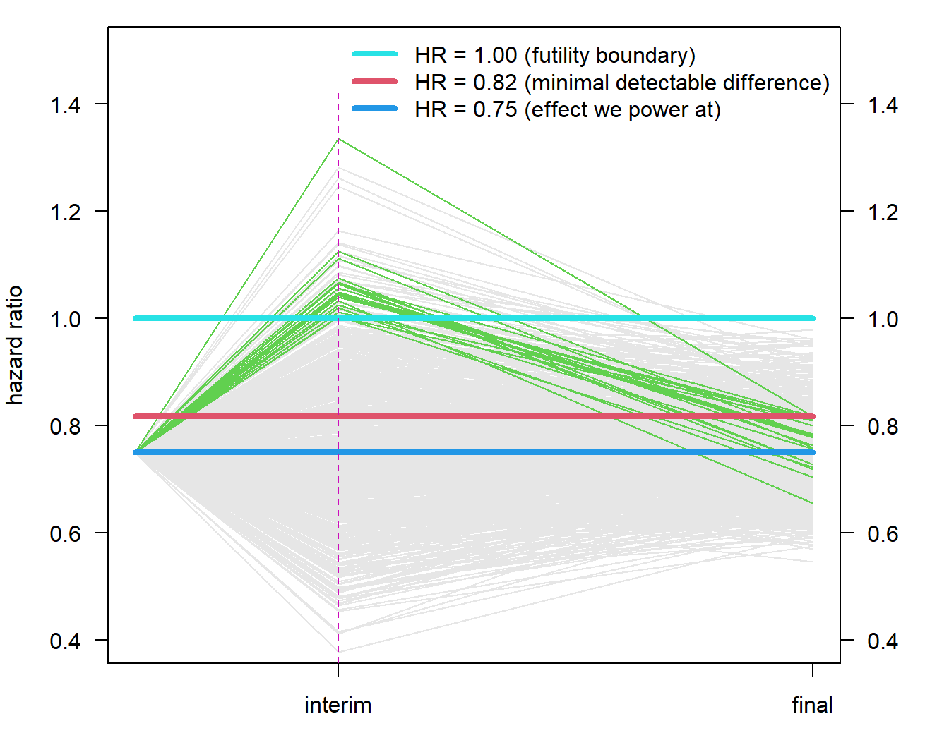
  legend("topright", paste("HR = ", disp(c(1, mdd_no_interim, hr), 2), " (", 
                           c("futility boundary", "minimal detectable difference", "effect we power at"), ")", 
                           sep = ""), bty = "n", lty = 1, col = c(5, 2, 4), lwd = 4)
  
  # vertical line
  if (vert){segments(inter_x[1], 0, inter_x[1], 1.42, lty = 2, col = 6)}
}

plot_empty <- function(){
  inter_x <- cutoff / max(cutoff)
  yli_traj <- c(0.4, 1.5)
  
  par(las = 1)
  par(mar = c(3, 4, 1, 4), las = 1)
  plot(0, 0, type = "n", xlim = c(0, 1), ylim = yli_traj, xlab = "", xaxt = "n", ylab = "hazard ratio")
  axis(side = 4, at = seq(0, 2, by = 0.2), labels = disp(seq(0, 2, by = 0.2), 1))
  axis(side = 1, at = inter_x[2], labels = c("interim", "final")[2])
}

Trial design

First, let us specify the basic parameters of a Phase 3 clinical trial with a time-to-event endpoint:

#  trial operating characteristics
alpha <- 0.05
beta <- 0.2

# exponential survival functions 
m1 <- 6 * 12
m2 <- 8 * 12
med <- c(m1, m2)

# effect to have 80% power at
hr <- m1 / m2

# accrual
recruit1 <- rep(25, 16)
recruit2 <- recruit1
recruit <- list(recruit1, recruit2)
n <- sum(unlist(recruit))
start.accrual <- c(0, 0)

# drop-out (2.5% annually)
dropout.year <- 0.025
dropout.month <- -log(1 - dropout.year) / 12
dropout <- rep(dropout.month, 2)

# cure proportion 
cure <- c(0, 0)

# We assume the shape parameter of the Weibull distribution is = 1.
# Compute the scale parameter corresponding to the above median for Exponential:
lambda <- log(2) / med
scale <- 1 / lambda

# specification of interim analysis
info_interim <- 0.3
futilityHR <- 0.9

So we plan a trial assuming:

• 1:1 randomization,
• a futility interim analysis after 30% of events,
• 80% power to
• detect a hazard ratio (HR) of 0.75
• using a two-sided logrank test
• with a significance level of 0.05.

Simulation of trials with and without futility interim analysis

We will simulate such trials to illustrate the false-positive risk of a futility interim. For the simulation we need to specify a few more quantities:

# Required events without interim
nevent <- getSampleSizeSurvival(lambda1 = getLambdaByMedian(m2), lambda2 = getLambdaByMedian(m1), 
                                sided = 1, alpha = alpha / 2, beta = beta)
mdd_no_interim <- nevent$criticalValuesEffectScale[1, 1]
nevent <- ceiling(nevent$maxNumberOfEvents)

# cutoffs
eventsInterim <- ceiling(info_interim * nevent)
cutoff <- c(eventsInterim, nevent)

# number of simulations
M <- 10 ^ 3

# now simulate trials and record hazard ratios at interim and final analysis cutoff
resHR <- data.frame(matrix(NA, nrow = M, ncol = length(cutoff)))
colnames(resHR) <- cutoff
resp <- resHR

for (i in 1:M){
  res2arm <- rWeibull2arm(scale = scale, shape = c(1, 1), 
                        cure = cure, recruit, dropout, start.accrual, cutoff, seed = NA)$tab

  for (j in 1:length(cutoff)){
    
    # compute hazard ratio for this cutoff
    tmt <- res2arm[, "tmt"]
    time <- res2arm[, paste("time cutoff = ", cutoff[j], sep = "")]
    event <- res2arm[, paste("event cutoff = ", cutoff[j], sep = "")]

    cox1 <- summary(coxph(Surv(time, event) ~ tmt))
    resHR[i, j] <- exp(coef(cox1)[1])
    resp[i, j] <- coef(cox1)[1, "Pr(>|z|)"]
  }
}

Quantification of power loss of interim analysis, and graphical illustration

We have now 1000 simulated trials with a hazard ratio estimate at the interim and final analysis. First, let us plot results assuming there would be no interim analysis. The horizontal lines correspond to the futility boundary, the minimal detectable difference (i.e. the hazard ratio we need to observe at the final analysis to be statistically significant), and the hazard ratio for which we specified the sample size to have 80% power at. They grey lines illustrate the hazard ratios we observe at the final analysis using these assumptions, with green lines those trials that would be statistically significant, i.e. land below the red horizontal line. These are 79.9% of trials (an estimate of the power).

plot_empty()

# plot trajectories to final only
segments(0, hr, 1, resHR[, 2], col = grey(0.9), lty = 1)

# significant trajectories
segments(0, hr, 1, resHR[resHR[, 2] <= mdd_no_interim, 2], col = 3, lty = 1)

horiz()

Now, we know that by adding a futility interim we reduce trial power, because we erroneously stop some trials that would be statistically significant at the final analysis. But how many? In order to find out we have to filter out those trials for which

• the hazard ratio at the interim analysis is above 1 (i.e. the interim boundary for futility) but
• below 0.818, i.e. the minimal detectable difference at the final analysis.

plot_empty()
inter_x <- cutoff / max(cutoff)
axis(side = 1, at = inter_x[1], labels = c("interim", "final")[1])

# all trajectories including interim
segments(0, hr, inter_x[1], resHR[, 1], col = grey(0.9), lty = 1)
segments(inter_x[1], resHR[, 1], 1, resHR[, 2], col = grey(0.9), lty = 1)

# color the false negatives: stopped at interim but sig at final
ind <- (resHR[, 1] > 1 & resHR[, 2] <= mdd_no_interim)
segments(0, hr, inter_x[1], resHR[ind, 1], col = 3, lty = 1)
segments(inter_x[1], resHR[ind, 1], 1, resHR[ind, 2], col = 3, lty = 1)

horiz(vert = TRUE)

The plot above indicates those 2.2% of trials that would be erronously stopped at the futility interim analysis. This is what is typically called the power loss of the futility interim analysis.